Getting Started
Overview
This document describes how to use the Galois system. Galois exploits the amorphous data-parallelism in iterative algorithms that manipulate dynamic data structures such as graphs and trees. The user expresses the algorithm using sequential Java code, but specifies the loops that contain parallelism using Galois Iterators. The resulting code has well-defined sequential semantics while allowing efficient parallelization.
Typically, an iterative algorithm obtains work items from a worklist and terminates once the worklist is empty. The processing of a work item may generate new work items that have to be added to the worklist. We refer to the node in the graph data structure that corresponds to a work item as an active node. We define active edges similarly but will ignore them in this document as they are treated in the same way as active nodes. The processing of an active node may touch other nodes (and edges) of the graph. This set of touched nodes is called the neighborhood of the active node. Figure 1 shows a sample graph with active nodes and their neighborhoods.
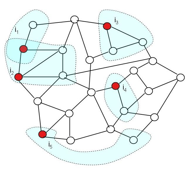
Figure 1: Graph with active nodes (red) and their neighborhoods (shaded blue regions).
In many algorithms, the order in which the active nodes are processed is irrelevant. In other algorithms, a partial or full order of processing active nodes must be followed. Aside from these ordering constraints (if any), it is easy to see from Figure 1 that active nodes can be processed in parallel as long as their neighborhoods do not overlap. In fact, even overlapping neighborhoods do not prevent parallel execution as long as the overlapped region is only read. Parallel execution is permissible in these cases because updates to the graph affect disjoint regions. Hence, the result of the parallel execution is identical to the result of a serial execution. We call this type of parallelism amorphous data-parallelism.
The current Galois release includes a dozen benchmarks representing important applications from a broad range of domains. These benchmarks are written in Java and use Galois extensions and classes, which are necessary for correct concurrent execution. This tool is work in progress and everything described herein is subject to change.
An Irregular Application: Spanning Tree Construction
We now illustrate the concepts on the example of building a spanning tree of a graph. Here, the worklist is initialized with a randomly selected node from the graph, which corresponds to the root of the spanning tree. The algorithm iteratively builds the spanning tree by growing a component C, which initially contains just the root node. At each point there is a set of edges connecting nodes inside C with the rest of the graph, thus defining a "cut". In each iteration the algorithm selects a node n from the worklist and for each cross-cutting edge of n, it adds the corresponding neighbor to C. Because at each point we can examine any cross-cutting edge to augment the spanning tree, there is no ordering constraint in the algorithm. A possible implementation of the algorithm is:
| 1 2 3 4 5 6 7 8 9 10 | Graph<NodeData> g = /* create graph instance */ Set<Edge> spanningTree = new HashSet<Edge>(); GNode<NodeData> root = g.getRandomNode(); addToTree(root); Set<GNode<NodeData>> ws = { root }; // populate workset with random root node while (!ws.isEmpty()) { GNode<NodeData> n = ws.removeAny(); // remove an element from the set ExpandTree(n, ws, spanningTree); // grow the tree } |
In line 1, the code instantiates the input graph g and populates it with nodes. In line 2 we create
a set that will hold the edges in the spanning tree. In lines 3-4, we
randomly select a node from the graph, add it to the spanning tree, and add it to a workset of nodes that need to be processed.
Finally, in lines 7-9 we keep expanding the tree by processing a random node from the workset. The loop terminates when
all nodes have been added to the spanning tree.
Galoizing a Java Program
Galois concepts
There are three steps that must be taken to convert a sequential Java program into a Galois compatible parallel program.
- The loop(s) that should be run in parallel must be written using
foreachconstructs. - The
foreachmust use one of the provided worklist classes. - The data structure(s) that will be accessed in parallel must be expressed using Galois-provided classes.
Conceptually, after performing these steps the parallel program looks as follows:
| 1 2 3 4 5 6 7 8 9 | Graph<NodeData> g = /* create graph instance */ Bag<Edge> spanningTree = new BagBuilder<Edge>().create() GNode<NodeData> root = g.getRandomNode(); addToTree(root); Worklist<GNode<NodeData>> ws = { root }; // populate workset with random root node foreach(GNode<NodeData> n : ws) { ExpandTree(n, ws, spanningTree); // grow the tree } |
The main changes are in lines 2, 4 and 6-8.
In line 2, we replace the Set type with a Bag type (provided by the Galois library),
which allows efficient concurrent additions.
In line 4, we create a Galois worklist, which we initialize with the root.
In lines 6-8, the sequential for loop over ws is replaced by a foreach loop.
In line 1 we use a Galois library provided implementation of Graph, which is "safe" for parallel execution.
Note that the code above presents the conceptual structure of the program. In the following section we describe how these concepts are implemented in
the Galois system.
Foreach loops and worklists
The Galois foreach loop is implemented as a call to the runtime library, which takes three arguments.
- A Java collection with the initial contents of the worklist.
- A function object representing the loop body.
- A set of rules that dictate the type and implementation of the worklist.
The actual source code for the above loop is provided below:
| 1 2 3 4 5 6 7 8 9 | GaloisRuntime.foreach( Arrays.asList(root), new Lambda2Void<GNode<NodeData>, ForeachContext<GNode<NodeData>>>() { public void call(GNode<NodeData> n, ForeachContext<GNode<NodeData>> worklist) { Expand(n, worklist, spanningTree); } }, Priority.defaultOrder() ); |
This code implements an unordered foreach loop.
In line 2, we provide the initial contents of the worklist in a collection initialized with root.
In lines 3-7 create a function object that implements the body of the parallel loop.
The method call takes two parameters: the first one (n) is the worklist
item that the current iteration is working on, and the second one (ctx) represents a handle
to the worklist. In line 8 we instruct the runtime to use the default implementation of a worklist that loosely
follows FIFO order for iterating over its contents.
For more information on these concepts, the reader is referred to the Foreach Usage and Tuning Hints sections.
Galois data structures
Galois programs must be careful about objects that could be accessed by two
different iterations of a foreach loop. Such objects need special,
data-structure specific logic to describe the relationship
between method calls and how to undo modifications to their
state. Currently, we provide a set of classes that are safe to
be shared between parallel iterations, including graphs and other collection classes. These classes are located
in the galois.objects package and its subpackages. Any
program that has shared objects that are not instances of these
classes will probably produce incorrect results when run concurrently.
Galois provides several graph
classes that share a common interface. For performance reasons, multiple graph classes are provided
that support different features, including directed and undirected edges, edges
with and without data, and graphs with indexed edges.
For the spanning tree example, the graph over which we build the spanning tree is implemented using
a general graph (galois.objects.graph.ObjectGraph).
An ObjectGraph has several concrete implementations that are appropriate for different types of applications.
In particular, the most general type is a MorphGraph, which allows adding and removing nodes and edges. There is also
a LocalComputationGraph that allows concurrent updates to the node and edge data, but not concurrent addition and removal of
nodes and edges. In this example, for simplicity, we will use a MorphGraph.
The graph of the spanning tree application does not require the existence of data on the edges.
To create an object of type MorphGraph without edges, we use a factory method provided by the class, as follows:
Graph<NodeData> graph = new MorphGraph.VoidGraphBuilder().directed(false).create();
Please refer to the galois.object.graph package for details about additional types of graphs and ways to build them.
Basic usage of the graph API
Below, we provide the implementation of the Expand method for the spanning tree example, which adds a new
edge to the tree.
| 1 2 3 4 5 6 7 8 9 10 11 12 13 14 15 | private void Expand(GNode<NodeData> n, ForeachContext<GNode<NodeData>> worklist, Bag<Edge> spanningTree) { n.map(new LambdaVoid<GNode<NodeData>>() { @Override public void call(final GNode<NodeData> dst) { //assume no self-edges NodeData dstData = dst.getData(); if (!dstData.inSpanningTree()) { Edge edge = new Edge(n, dst); spanningTree.add(edge); dstData.setInSpanningTree(true); worklist.add(dst); } } }); } |
The Expand method above expects three parameters, namely the current worklist element n,
the worklist handle, and the spanningTree that we are augmenting.
Expand augments the spanningTree by checking each neighbor of n individually
and adding it to the tree if it is not already there.
To perform a specific action on each of the neighbors of n, in line 2 we invoke the map method,
which takes as an argument a function object that contains the operation that is to be applied to each individual neighbor.
The type of the function object, LambdaVoid, is provided by the Galois library and represents a function with
a single argument, and no return value. In lines 6-7, we examine whether the data item associated with the neighbor
node dst is already in the tree. If not, in lines 8-10, we create an edge (represented simply as an unordered pair)
that connects the two nodes, add it to the spanning tree, and mark dst as a node of the tree. Finally, in line 11,
we add dst to the worklist for further processing by subsequent iterations of the foreach loop.
Controlling conflict detection
Each call to Expand visits the neighbors of a node, examines the value of their data, potentially modifies the data of some
neighboring nodes, and updates the collection of tree edges. By default, an iteration calling a graph method acquires ownership of the nodes
and edges the method manipulates, and also saves undo information when needed. Calls to other Galois collections, such as Bag, behave similarly. The Galois library provides the abstract implementation galois.objects.AbstractBaseObject that
can be extended by application-level types. It implements a simple exclusive locking policy with rollbacks implemented by copying.
Therefore, in the code above, each iteration will try to acquire ownership of n, all its neighbors, and their corresponding data.
In addition, for each modification made to user data, the iteration must store appropriate information in order to be able to undo the speculative
side-effects of actions it performs. Such actions usually have a performance impact and reduce the amount of extracted parallelism.
The following simple observations help us optimize the above mentioned overheads. First, by calling map an iteration acquires
ownership on each neighbor of n. Therefore, subsequent calls that refer to those nodes, such as the call in line 6, can skip this task. Additionally, since each node has its own private data item, protecting the node effectively protects its associated data item too. Finally, in lines 9-11 where Expand updates the collection of tree edges and the worklist, the iteration cannot fail anymore and
is no longer considered speculative. As a result, no undo information needs to be stored in lines 9 and 11.
The implementation allows an optional parameter, MethodFlag.NONE,
to Galois collection methods that avoids all of the above mentioned overheads. The optimized version of the method is provided below.
| 1 2 3 4 5 6 7 8 9 10 11 12 13 14 15 | private void Expand(GNode<NodeData> n, ForeachContext<GNode<NodeData>> worklist, Bag<Edge> spanningTree) { n.map(new LambdaVoid<GNode<NodeData>>() { @Override public void call(final GNode<NodeData> dst) { //assume no self-edges NodeData dstData = dst.getData(MethodFlag.NONE); if (!dstData.inSpanningTree()) { Edge edge = new Edge(n, dst); spanningTree.add(edge, MethodFlag.NONE); dstData.setInSpanningTree(true); worklist.add(dst, MethodFlag.NONE); } } }); } |
For a full list of available flags to control the Galois collection methods,
the reader is referred to the galois.objects.MethodFlag class and the Tuning Hints section.
Compiling and Running a Galois Program
Directory structure
The directory structure of the Galois distribution is as follows:
All applications written for Galois must reside in the apps directory in order to
be correctly compiled by the system. The complete spanning tree source code is in the apps/spanningtree/main/ directory.
Application-specific parameters including command-line arguments are contained in the conf directory.
The parameters are stored in standard Java properties file format. Command-line arguments are specified
by the value of the args key in the properties file. For example,
the spanning tree's small.properties file contains the following line, which indicates a random input graph of 800,000 nodes, with
each node having between 5 and 10 neighbors:
Compiling and running the spanning tree application
To compile the spanning tree application the user should execute the following command in the Galois root directory.
This command invokes the ant build script and instructs to compile the application located in apps/spanningtree, along with
the rest of the Galois runtime system. Upon successful completion, the generated class files appear inside the classes directory.
To run the spanning application, the user should execute the following command in the Galois root directory.
Here we invoke the application spanningtree.main.Main with input arguments residing in the file apps/spanningtree/conf/medium.properties.
We use 2 threads, 2 GB of heap space, and execute the application 3 times inside the same JVM instance. The input arguments can be specified at the command line instead of an input file. For more detail on the usage of this script, please see the Command Line section.
Executing the above command should generate output that looks as follows:
The output shows the execution times (in milliseconds) for each of the three runs of the application (both with and without garbage collection time). At the end it prints out some Galois system statistics, including the abort ratio, the number of committed and total iterations, and some execution time statistics after dropping the first experiment (to preclude JIT compilation related side-effects). For more detail, please see the Command Line section.
Profiling with ParaMeter
Galoised applications can be profiled with the ParaMeter profiling tool that is included in the release. To generate a ParaMeter profile and statistics for our spanning-tree sample application for a run with the medium input, simply execute the following command in the Galois base directory:
Running this command generates the file parameterStats.csv in the current directory, which contains the raw ParaMeter output in comma-separated value format. If the R statistics package is installed, the parameter script will output several summarizing graphs to the file parameterProfile.pdf.
The output includes, for each time step, the number of active nodes, the worklist size at the beginning of each time step, the number of active nodes that were invalidated by previous work (i.e., "not useful" work), as well as the average, minimum, and maximum neighborhood size and the standard deviation thereof. The neighborhood size is measured by the number of logical locks acquired during an iteration of a foreach loop. Logical locks are acquired for each shared object that implements the Lockable interface, subjects to the method flags. Thus, the neighborhood size is the sum over all shared objects that were locked by an iteration.
ParaMeter output
Figure 2 depicts the first graph generated by ParaMeter. The curve in blue shows the number of active nodes successfully processed in each time step, called the available parallelism. The black line indicates the average over all time steps. The exponential increase in parallel work matches our intuition about building a spanning tree of a random graph in which each node has between five and ten neighbors. Initially, the tree is small and there is only little work on the worklist, which limits parallelism. As the tree grows, more and more (largely independent) work is added. Correspondingly, the amount of parallel work rapidly increases until the algorithm starts running out of work.
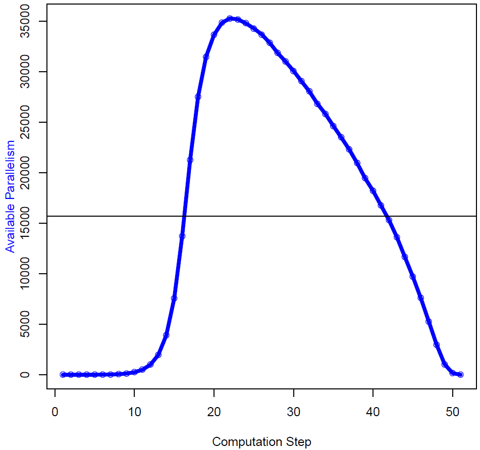
Figure 2: Available parallelism profile of the spanning tree code.
Figure 3 shows the second graph generated by ParaMeter. It again shows the available parallelism in blue but also a black curve that indicates the total number of activities on the worklist (the worklist size), the parallelism intensity in green (which is the available parallelism divided by the worklist size), the amount of new work added in violet, and the amount of useless work in red. Note that the scale for the parallelism intensity is to the right. In case of the spanning-tree example, there is no useless work.
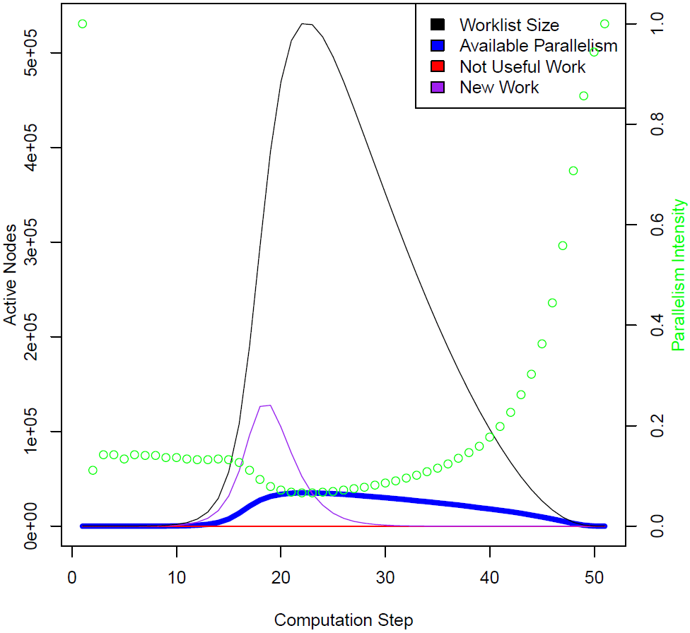
Figure 3: Parallelism intensity profile of the spanning tree code.
Figure 4 shows the third graph generated by ParaMeter. It once again shows the available parallelism in blue, this time augmented with the minimum, mean, and maximum neighborhood sizes in violet, black, and red, respectively. Note that the scale for the neighborhood sizes is to the right.
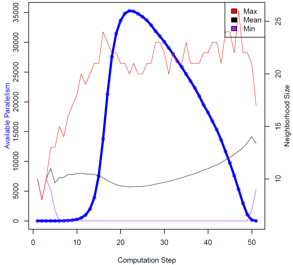
Figure 4: Neighborhood profile of the spanning tree code.