GMetis
Application Description
This benchmark produces a k-way partitioning of a graph. It implements the algorithm proposed by George Karypis and Vipin Kumar [1]. The data parallelism in this algorithm arises from the nodes of the graph that can be processed in parallel (including matching, adding neighbors, and moving nodes).
[1] Multilevel k-way Partitioning Scheme for Irregular Graphs. George Karypis and Vipin Kumar. J. Parallel Distrib. Comput. 48(1): 96-129, 1998.
Algorithm
GMetis is a multilevel partitioning algorithm. It first iteratively coarsens the graph by collapsing nodes until the graph is small enough, then it uses PMetis (a multilevel recursive bisection algorithm) to produce a k-way partitioning of the small graph, and finally it projects the partitioning back to the original graph. During each projection to the next finer graph, it refines the partitioning.
| 1 2 3 4 5 6 7 8 9 10 11 12 13 14 15 16 17 | Graph g = /* read in graph */; int k = /* num of partitions */; Graph original = g; do { Match m = g.match(); Graph cg = g.createCoarseGraph(m); cg.setFinerGraph(g); g = cg; } while (!g.coarseEnough()); PMetis.partition(g, k); while (g != original){ Graph fg = g.getFinerGraph(); g.projectPartitioning(fg); fg.computeInfoForRefining(); fg.randomRefine(); g = fg; } |
Figure 1: Pseudocode for GMetis.
| 1 2 3 4 5 | foreach (Node n : graph) { // randomly access if (n.isMatched()) continue; Node match = n.getUnmatchedNeighborWithMaxEdgeWeight(); graph.setMatch(n, match); } |
Figure 2: Pseudocode for g.match() using heavy edge matching.
| 1 2 3 4 5 6 7 8 9 10 11 12 13 14 15 16 17 18 19 20 21 22 23 24 | Graph cg = new Graph(); // Coarse Graph for (Node n : graph) { if (n.visited) continue; Node cn = cg.createNode(); n.setRepresentative(cn); n.getMatch().setRepresentative(cn); n.getMatch().setVisited(true); } //reset visited field for each node in the graph ... foreach (Node n : graph) { if (n.visited) continue; // add edges in cg according to n's neighbors for (Node nn : n.getNeighbors()) { Edge e = graph.getNeighbor(n, nn); Node cn = n.getRepresentative(); Node cnn = nn.getRepresentative(); Edge ce = cg.getEdge(cn, cnn); if (ce == null) { cg.addEdge(cn, cnn, e.getWeight()); } else { ce.increaseWeight(e.getWeight()); } // add edges in cg according to n.getMatch()'s neighbors, similar to n ... n.getMatch().setVisited(true); } } |
Figure 3: Pseudocode for Create Coarse Graph.
| 1 2 3 4 | foreach (Node n : graph.boundaryNodes()) { n.computeInternalDegree(); n.computeExternalDegree(); } |
Figure 4: Pseudocode for Compute Info For Refining.
| 1 2 3 4 5 6 7 8 9 | Workset ws = new Workset(); foreach (Node n : graph.boundaryNodes()) { if (/* moving n to neighbor partition reduces graphcut */) ws.add(n); } foreach (Node n : ws) { if (/* balancingCondition is not violated */) moveNode(n); } |
Figure 5: Pseudocode for Random K-Way Refinement.
In more detail, the algorithm proceeds as follows: (pseudocode is provided in Figure 1). The algorithm consists of three phases: coarsening (line 4-9 in Figure 1), initial partitioning (line 10 in Figure 1), and projection & refining (line 11-17 in Figure 1). In coarsening, it iteratively coarsens the graph into a smaller graph until the graph is small enough (line 9 in Figure 1). In each iteration, two steps are performed: matching (line 5 in Figure 1) and creating the coarser graph (line 6 in Figure 1). Matching matches each node in the graph with one of its unmatched neighbors (if there is no such neighbor, the node matches itself). Here a heuristics called "heavy edge matching" is used (Figure 2). Heavy edge matching (HEM) works as follows: the nodes in the graph are visited randomly (allowing the use of an unordered worklist) and each node is matched to the neighbor with the maximal edge weight among all of its unmatched neighbors. If there is no such neighbor, the node matches itself. Creating the coarse graph is done by collapsing the matched node pairs. Note that the collapsing is not done in place; instead, a list of graphs is kept (line 7 in Figure 1). The pseudocode for creating a coarse graph can be found in Figure 3.
For the initial partitioning, PMetis is used to partition the coarsest graph into k partitions. PMetis is a serial recursive multilevel bisection algorithm [2]. In the projection & refining phase, the partitioning of a graph is iteratively projected back to the next finer graph (line 13 in Figure 1) until the original graph is reached. In each iteration, after projecting the partitioning, the partitioning is refined (line 15 in Figure 1). A random k-way refinement algorithm is used here: each boundary node under the current partitioning is moved to a neighbor partition of its current partition if moving it to that partition reduces the graph cut and does not make the partitioning unbalanced. If there are multiple neighbor partitions to move to, the one that reduces the graph cut the most is chosen. The boundary nodes are visited randomly, so an unordered worklist is used. The pseudocode for random refinement can be found in Figure 5. The refinement algorithm needs to use the internal and external degree of each node in the graph. This information is computed before the start of the refinement algorithm(line 14 in Figure 1). The pseudocode for Computing Informaton For Refinement can found in figure 4.
[2] A fast and high quality multilevel scheme for partitioning irregular graphs. George Karypis and Vipin Kumar. International Conference on Parallel Processing, pp. 113-122, 1995
Data Structures
There are two key data structures used in GMetis:
- Unordered Set
- The worklist used to hold the graph nodes is represented as an unordered set.
- Graph
- A directed graph data structure is used to represent the undirected input graph, in which every node and every edge stores weights.
Parallelism
All the foreach loops in the various algorithm components can be parallelized. In the matching step, if two nodes in the graph do not share neighbors, they can be processed in parallel. Since the input for the GMetis algorithm is usually a large sparse graph, the parallelism is often large. In the coarsening step, there is also a lot of parallelism. If two representative nodes in the coarser graph are not neighbors, their edges can be added in parallel. In the refinement step, if two boundary nodes do not share neighbors, they can be moved in parallel. In the step that computes information for refinement, every node in the graph reads the partitions of neighbor nodes and writes its internal and external degree, so this step is a reader and there are no conflicts.
The available parallelism of the foreach loops in GMetis is shown in Figure 6. The input has 60,005 nodes and 89,440 edges.
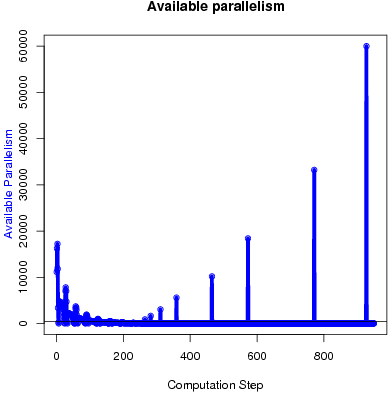
Figure 6: Available parallelism in GMetis.
Performance
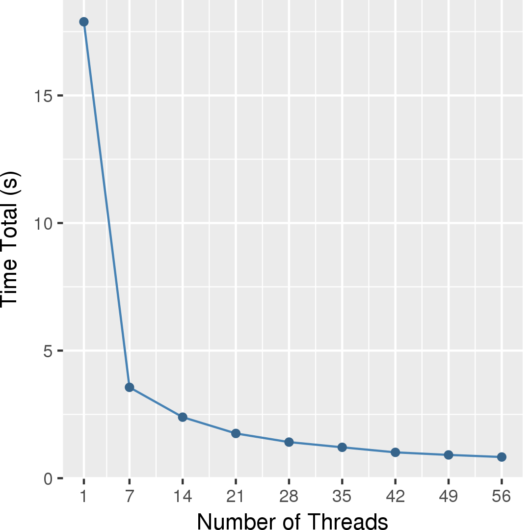
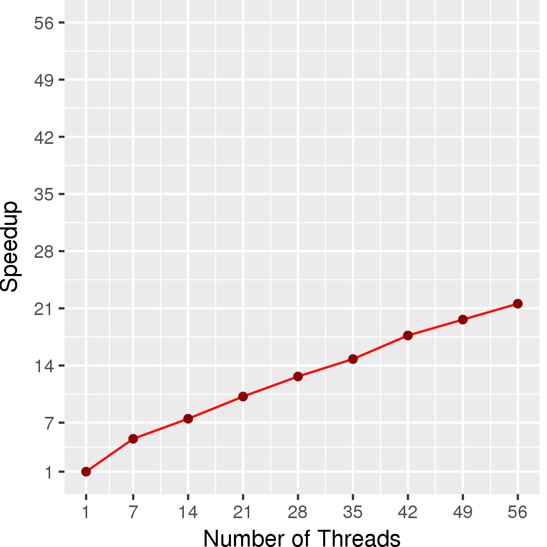
Figure 7 and Figure 8 show the total running time in seconds and self-relative speedup (speedup with respect to the single thread performance), respectively, of GMetis for an input graph with 5,154,859 nodes and 47,022,346 edges. The total running time measured is spent in the whole partitioning phase consisting of serial phases and parallel phases.
Machine Description
Performance numbers are collected on a 4 package (14 cores per package) Intel(R) Xeon(R) Gold 5120 CPU machine at 2.20GHz from 1 thread to 56 threads in increments of 7 threads. The machine has 192GB of RAM. The operating system is CentOS Linux release 7.5.1804. All runs of the Galois benchmarks used gcc/g++ 7.2 to compile.