Betweenness Centrality
Application Description
This benchmark computes the betweenness centrality of each node in a network, a metric that captures the importance of each individual node in the overall network structure. Betweenness centrality is a shortest path enumeration-based metric. Informally, it is defined as follows. Let \(G=(V,E)\) be a graph and let \(s,t\) be a fixed pair of graph nodes.The betweenness score of a node \(u\) is the percentage of shortest paths between \(s\) and \(t\) that include \(u\). The betweenness centrality of \(u\) is the sum of its betweenness scores for all possible pairs of \(s\) and \(t\) in the graph. The benchmark takes as input a directed graph and returns the betweenness centrality value of each node.
We have two different implementations: one that we term outer betweenness centrality and the BC algorithm presented by Dimitrios Prountzos. Both are based upon Brandes's algorithm which we present here.
Brandes's Algorithm
Our parallel implementations are based on Brandes's algorithm [1]. Brandes's algorithm exploits the sparse nature of typical real-world graphs, and computes the betweenness centrality score for all vertices in the graph in \(O(VE + V^2 \log{V})\) time for weighted graphs, and \(O(VE)\) time for unweighted graphs. The current implementations deal only with unweighted graphs.
Formally, let \(G=(V,E)\) be a graph and let \(s,t\) be a fixed pair of graph nodes. Let \(\sigma_{st}\) be the number of shortest paths between \(s\) and \(t\), and let \(\sigma_{st}(v)\) be the number of those shortest paths that pass through \(v\). We define the dependency of a source vertex \(s\) on a vertex \(v\) as: \[ \delta_{s}(v) = \sum_{t \in V} \frac{\sigma_{st}(v)}{\sigma_{st}} \] This dependency captures the importance of the node with respect to \(s\) and \(t\). The betweenness centrality of a vertex \(v\) is then expressed as: \[ BC(v) = \sum_{s \neq v \in V} \delta_{s}(v) \] The key insight is that the dependency of a node \(v\) satisfies the following recurrence: \[ \delta_{s}(v) = \sum_{w \colon v \in pred(s,w)} \frac{\sigma_{sv}}{\sigma_{sw}}(1 + \delta_{s}(w)) \] where \(pred(s,w)\) is the set of predecessors of \(w\) in the shortest paths from \(s\) to \(w\).
Using this insight, Brandes's algorithm works as follows: Initially, \(V\) shortest-path computations are done, one for each \(s \in V\). In the case of unweighted graphs, these shortest path computations correspond to breadth-first search (BFS) explorations. The predecessor sets \(pred(s,v)\), and \(\sigma_{sv}\) values are computed during these shortest-path explorations. Next, for every possible source \(s\), using the information from the shortest paths tree and the DAG that is induced on the graph by the predecessor sets, we compute the dependencies \(\delta_{s}(v)\) for all other \(v \in V\). To compute the centrality value of a node \(v\), we finally compute the sum of all dependency values.
This algorithm has parallelism at multiple levels. Firstly, we can perform the shortest path exploration from each source node in parallel. Additionally, each of the shortest path computations can be done in parallel.
Outer Betweenness Centrality
Outer Betweenness Centrality exploits parallelism using the former approach. Different threads execute single shortest-path computations independently, and they use that information to compute the contribution from each individual source to the betweenness centrality of each node in the graph. The process is described in Figure 1.
| 1 2 3 4 5 6 7 8 9 10 | Graph g = /* read input graph */; Workset ws = new Workset(g.getNodes()) foreach (Node s : ws) { Perform forward BFS: compute BFS DAG for all nodes compute \(\sigma_{sv}\) For all nodes \(v\) in the BFS DAG: compute \(\delta_{s}(v)\) \(BC(v) += \delta_{s}(v)\) } |
Figure 1: Pseudocode for Outer Betweenness Centrality.
One thing to note is that, with the exception of line 9, the computations performed by different iterations are independent. This requires the use of thread local storage on each thread to keep its calculations independent. The updates to the betweenness values in line 8 are simple reductions and do not generate conflicts. Additionally, since this algorithm is compute-intensive, even for relatively small graphs, we can compute an approximation of the betweenness value by populating the worklist (line 2) with only a subset of the graph nodes as shortest-path sources.
Asynchronous Brandes Betweenness Centrality
Our second implementation takes advantage of parallelism at the inner level (the shortest path and dependencies computations themselves rather than each source node). The algorithm is the one presented by Prountzos and Pingali [3]: it is a formulation of Brandes's algorithm under the operator formulation of algorithms.
Nodes are added to a worklist when work needs to be done, and the parallelism occurs here where threads will take items from the worklist and work on them independently. When a thread takes an item from a worklist, it does a series of condition checks on the data stored in the node and its neighbors/edges to determine which operator needs to be applied. The operator will update the node state and potentially push other nodes onto the worklist. There are two separate phases for the algorithm for each source handled. The first will determine the shortest-path counts and distances for the source node that is being worked on. This, as a result, will construct a shortest-path DAG. The second will propagate dependencies starting from the leaves of the DAG. Each phase has its own set of operators to be applied to worklist items to progress computation.
| 1 2 3 4 5 6 7 8 9 10 11 12 13 14 15 16 17 18 19 20 21 22 23 24 25 | Graph g = /* read input graph */; for (node n in graph g) { Initialize n as source node for BC Worklist wl1 = new Worklist with only n // construct DAG foreach (node s in wl1) { // operators can add items to wl1 for (each edge in s) { check nodes and edges to see if any operator can be applied } } Worklist wl2 = new Worklist with nodes that have no successors in DAG // propagate dependencies backward from DAG foreach (node s in wl2) { update s's predecessors p by pushing out dependency and add p to wl2 if p has no more unprocessed successors } for all nodes except n { add dependency to current BC value } } |
Figure 2: Pseudocode for Asynchronous Brandes Betweenness Centrality.
This algorithm is known to perform very well on road network-like graphs.
For more details on the operators and the algorithm itself, please refer to the PPoPP'13 paper [3].
Performance
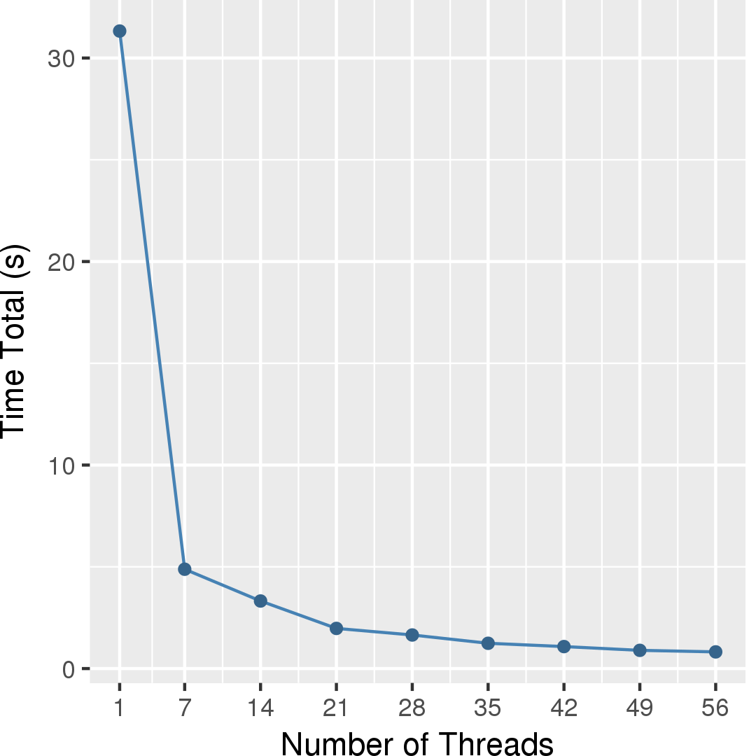
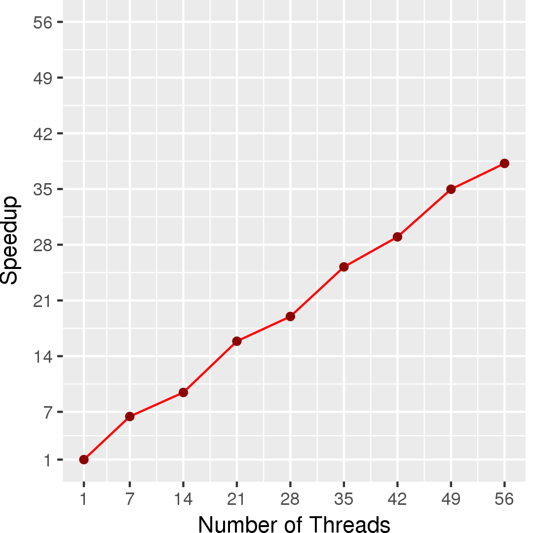
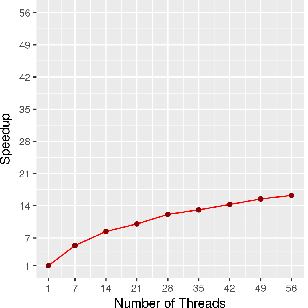
Figure 3 and Figure 4 show the execution time in seconds and self-relative speedup (speedup with respect to the single thread performance), respectively, of the outer BC algorithm running on a graph generated using rmat model with 2^14 nodes and 2^17 edges. Similarly, Figure 5 and Figure 6 show the execution time in seconds and self-relative speedup, respectively, of the asynchronous Brandes BC algorithm running on the USA road network from 5 source nodes.

[1] Ulrik Brandes: A Faster Algorithm for Betweenness Centrality, Journal of Mathematical Sociology 2001.
[2] http://www.graphanalysis.org/benchmark/
[3] D. Prountzos and K. Pingali. Betweenness centrality: algorithms and implementations, PPoPP 2013.
[4] D. Chakrabarti, Y. Zhan, and C. Faloutsos, R-MAT: A recursive model for graph mining, SIAM Data Mining 2004.
Machine Description
Performance numbers are collected on a 4 package (14 cores per package) Intel(R) Xeon(R) Gold 5120 CPU machine at 2.20GHz from 1 thread to 56 threads in increments of 7 threads. The machine has 192GB of RAM. The operating system is CentOS Linux release 7.5.1804. All runs of the Galois benchmarks used gcc/g++ 7.2 to compile.