Minimum Weight Spanning Tree
Application Description
The Spanning Tree of an undirected graph is an acyclic subset of the graph's edges that connects all of the vertices belonging to the graph. In the graph's edges are labeled with weights, the the Minimum Weight Spanning Tree (MST) is a spanning tree that has the minimum sum of edge weights. In the following, we briefly describe Boruvka's algorithm.
Boruvka's Algorithm
Boruvka's algorithm [1] computes the minimal spanning tree through successive applications of edge-contraction on an input graph (without self-loops). In edge-contraction, an edge is chosen from the graph and a new node is formed with the union of the connectivity of the incident nodes of the chosen edge. In the case that there are duplicate edges, only the one with least weight is carried through in the union. Figure 1 demonstrates this process. Boruvka's algorithm proceeds in an unordered fashion. Each node performs edge contraction with its lightest neighbor. This is in contrast with Kruskal's algorithm where, conceptually, edge-contractions are performed in increasing weight order.
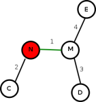
Figure 1a: Before edge-contract.
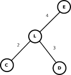
Figure 1b: After edge-contract.
While in principle, the edge-contraction operation can be performed by modifying the graph, it is costly to implement. Most implementations use a Union-Find (aka Disjoint-Set [2]) data structure, instead, to perform edge-contractions. Union-Find data structure assigns a unique component to each node; a component is identified by its representative, which initially is the node itself. Every node in the component has a (direct or indirect) reference to its representative. The algorithm uses a Find operation to find the representative of the component the node belongs to. If the two nodes of the lightest edge point to different representatives, then they must belong to different components and adding the edge to the MST does not introduce a cycle. Adding an edge to the MST involves combining the two components (to which the two nodes of the edge belong to) into one component. This is done by performing a Union operation on the representatives of the two components, which essentially makes one representative point to the other. Figure 2 gives the pseudocode for Boruvka's algorithm:
| 1 2 3 4 5 6 7 8 9 10 11 12 13 | Graph g = /* read input */; UnionFind uf (g.getNodes ()); Workset ws = g.getNodes(); foreach (Node n : ws) { Edge e = minWeight (g.getOutEdges (n)); Node rep1 = uf.find (e.src); Node rep2 = uf.find (e.dst); if (rep1 != rep2) { e.markInMST(); Node rep = uf.union (rep1, rep2); ws.add (rep) } } |
Figure 2: Pseudocode for Boruvka's algorithm.
Data Structures
There are three key data structures used in Boruvka's algorithm:
- Graph
- The input, which is a weighted, undirected graph.
- Unordered Set
- The workset containing representative nodes
- Union-Find
- A disjoint-set data structure used to maintain components of graph.
Parallelism
Initially, there is a lot of parallelism in Boruvka's algorithm as about half the nodes can perform edge-contraction independently. After edge-contraction, the graph becomes more dense and there are fewer nodes, so the available parallelism decreases quickly. Figure 3 shows the parallelism profile for a sample input. Most parallel implementations of minimal spanning tree algorithms begin with Boruvka's algorithm but switch to another algorithm as the graph becomes more dense.
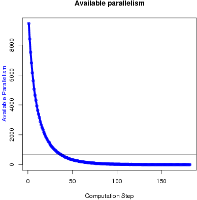
Figure 3: Available parallelism in Boruvka's algorithm.
Performance
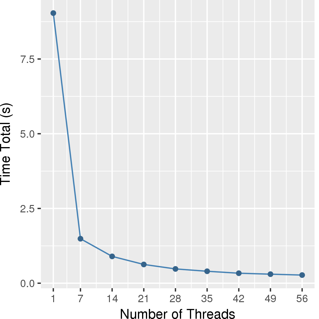
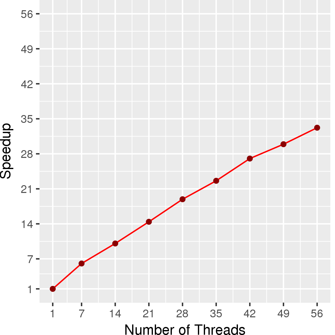
In our implementation of Boruvka, we split the loop body into two parallel phases, which have a barrier in between them. The first phase invokes Find on the lightest edge of each representative, while the second phase performs Union operation. The tresulting set of representatives is then used for the next round in a similar manner. This makes the concurrency control of UnionFind data structure simpler, where one of the costly and complex mechanism is finding conflicts between concurrent Union and Find operations. With splitting into phases, Find operations can proceed in parallel with Find operations (conceptually being readonly). Similarly Union operations on separate compononets can proceed in parallel without any concurrency control.Figure 4 and Figure 5 show the execution time in seconds and self-relative speedup (speedup with respect to the single thread performance), respectively, of Boruvka's algorithm on the USA road network.
[1] http://en.wikipedia.org/wiki/Boruvka's_algorithm
[2] Thomas H. Cormen, Charles E. Leiserson, Ronald L. Rivest, Clifford Stein.
Introduction to Algorithms. 2nd Edition, MIT Press, 2001.
Machine Description
Performance numbers are collected on a 4 package (14 cores per package) Intel(R) Xeon(R) Gold 5120 CPU machine at 2.20GHz from 1 thread to 56 threads in increments of 7 threads. The machine has 192GB of RAM. The operating system is CentOS Linux release 7.5.1804. All runs of the Galois benchmarks used gcc/g++ 7.2 to compile.